Deep Learning Models A Comprehensive Overview

Deep learning models are revolutionizing numerous fields, from image recognition to autonomous vehicles. This exploration delves into the core concepts, architectures, training methods, and applications of these powerful tools. We will examine various deep learning architectures, including convolutional neural networks (CNNs), recurrent neural networks (RNNs), and generative adversarial networks (GANs), highlighting their unique capabilities and real-world impact. The journey will cover the historical evolution of deep learning, the intricacies of model training, and the crucial aspects of model evaluation.

Finally, we will discuss future trends and ethical considerations within this rapidly advancing field.

Understanding deep learning requires a grasp of its fundamental building blocks and how they interact to produce sophisticated results. We’ll unpack the mechanics of backpropagation, the optimization algorithms used for fine-tuning model parameters, and common challenges such as overfitting and vanishing gradients. Through illustrative examples and case studies, we aim to provide a clear and accessible understanding of this transformative technology.

Introduction to Deep Learning Models

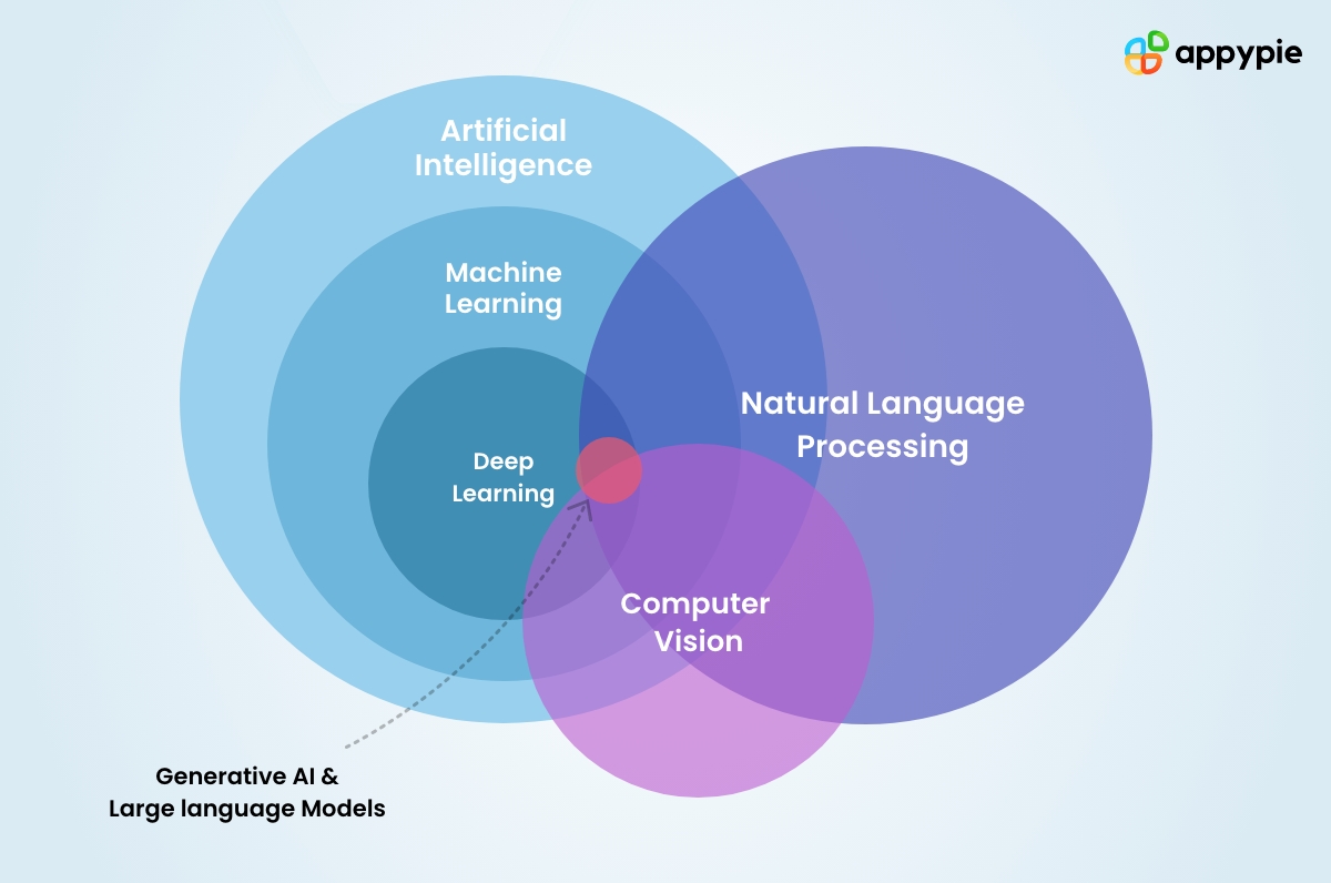
Deep learning, a subfield of machine learning and artificial intelligence (AI), focuses on algorithms inspired by the structure and function of the brain called artificial neural networks. These networks consist of multiple layers, allowing them to learn complex patterns and representations from data. Unlike traditional machine learning, deep learning excels at automatically extracting features from raw data, reducing the need for extensive manual feature engineering.

This capability makes it particularly powerful for handling large and complex datasets.Deep learning’s relationship to AI is that it’s a powerful tool within the broader field. AI aims to create intelligent systems, and deep learning provides a specific set of techniques for achieving this, particularly in tasks involving pattern recognition, prediction, and decision-making.

A Brief History of Deep Learning

The conceptual foundations of deep learning were laid in the mid-20th century with the development of the perceptron, a simple artificial neuron. However, early neural networks were limited by computational constraints and the lack of sufficient data. Significant advancements came in the late 2000s and early 2010s with increased computational power (especially GPUs), the availability of massive datasets, and the development of more sophisticated algorithms like backpropagation and dropout.

These breakthroughs led to a resurgence of interest in deep learning, resulting in significant improvements in various fields. The ImageNet competition, starting in 2010, served as a crucial benchmark, showcasing the dramatic performance improvements achieved by deep learning models compared to traditional methods.

Examples of Deep Learning Architectures

Deep learning encompasses a wide range of architectures, each designed for specific tasks. The choice of architecture depends on the nature of the data and the problem being addressed. Below is a table outlining some key architectures and their applications.

Architecture	Description	Applications	Example
Convolutional Neural Networks (CNNs)	Specialized for processing grid-like data such as images and videos. They use convolutional layers to extract features from local regions of the input.	Image classification, object detection, image segmentation, video analysis	Identifying cats and dogs in images; detecting cancerous cells in medical scans.
Recurrent Neural Networks (RNNs)	Designed to handle sequential data like text and time series. They have internal memory that allows them to process information over time. Long Short-Term Memory (LSTM) and Gated Recurrent Unit (GRU) are popular variations that address the vanishing gradient problem.	Natural language processing (NLP), machine translation, speech recognition, time series forecasting	Translating English text to French; predicting stock prices.
Generative Adversarial Networks (GANs)	Composed of two networks: a generator that creates synthetic data and a discriminator that tries to distinguish between real and synthetic data. They are trained in a competitive manner, leading to the generator producing increasingly realistic data.	Image generation, drug discovery, style transfer, data augmentation	Generating realistic images of faces; creating new drug molecules; converting a painting to the style of Van Gogh.
Autoencoders	Used for dimensionality reduction and feature extraction. They consist of an encoder that compresses the input data and a decoder that reconstructs the input from the compressed representation.	Anomaly detection, image denoising, data compression	Identifying fraudulent credit card transactions; removing noise from images.

Architectures of Deep Learning Models

Deep learning models are not monolithic; rather, they exhibit a diverse range of architectures, each tailored to specific tasks and data types. Understanding these architectural differences is crucial for effectively applying deep learning techniques. This section delves into the inner workings of several prominent architectures, highlighting their key components and functionalities.

Convolutional Neural Networks (CNNs)

Convolutional Neural Networks are particularly well-suited for processing grid-like data, such as images and videos. Their architecture leverages convolutional layers, pooling layers, and fully connected layers to extract features and make predictions.Convolutional layers employ filters (kernels) that slide across the input data, performing element-wise multiplication and summation to produce feature maps. These feature maps highlight specific patterns within the input.

For example, in image recognition, a filter might detect edges or corners. The process is repeated with multiple filters, each detecting different features. The number of filters determines the depth of the resulting feature maps.Pooling layers reduce the dimensionality of the feature maps, making the network less sensitive to small variations in the input and reducing computational complexity.

Common pooling operations include max pooling (selecting the maximum value within a region) and average pooling (averaging the values within a region). This downsampling helps to capture the most salient features while discarding less important details.Fully connected layers are located at the end of the CNN architecture. They receive the flattened output from the pooling layers and perform a standard feed-forward operation, mapping the extracted features to the desired output.

For instance, in a classification task, the output layer would have nodes representing different classes, with each node’s activation indicating the probability of the input belonging to that class. This final layer combines the information extracted from the previous layers to make a final decision.

Recurrent Neural Networks (RNNs): LSTMs and GRUs

Recurrent Neural Networks are designed to process sequential data, such as text and time series. Unlike feedforward networks, RNNs possess loops that allow information to persist across time steps. However, standard RNNs suffer from the vanishing gradient problem, which limits their ability to learn long-range dependencies. Long Short-Term Memory (LSTM) networks and Gated Recurrent Units (GRUs) address this limitation through sophisticated gating mechanisms.LSTMs utilize three gates: an input gate, a forget gate, and an output gate.

These gates control the flow of information into, out of, and within the cell state, allowing the network to selectively remember or forget information over time. This selective memory mechanism enables LSTMs to capture long-range dependencies more effectively than standard RNNs. For example, in natural language processing, an LSTM can effectively capture the context of a word even if it is separated from other related words by a long sequence of intervening words.GRUs, a simpler variant of LSTMs, combine the forget and input gates into a single update gate.

This simplification reduces the number of parameters and computational cost compared to LSTMs, while still maintaining good performance in many applications. While slightly less expressive than LSTMs, GRUs often demonstrate faster training times and can be preferable when computational resources are limited. Both LSTMs and GRUs have proven effective in various applications, including machine translation, speech recognition, and time series forecasting.

Generative Adversarial Networks (GANs)

A Generative Adversarial Network (GAN) consists of two neural networks: a generator and a discriminator. The generator creates synthetic data samples, while the discriminator attempts to distinguish between real and generated samples. This adversarial training process drives both networks to improve their performance.[Diagram description: The diagram shows two neural networks, the generator and the discriminator, connected in a loop.

Arrows indicate the flow of information. The generator takes random noise as input and produces synthetic data. This synthetic data is fed into the discriminator, along with real data samples. The discriminator outputs a probability indicating whether the input is real or fake. The discriminator’s output is used to train both the generator and the discriminator through backpropagation.

The generator aims to produce samples that fool the discriminator, while the discriminator aims to accurately classify real and fake samples. This adversarial process leads to an improvement in the generator’s ability to produce realistic data.]

Training Deep Learning Models

Training a deep learning model involves iteratively adjusting its internal parameters to minimize the difference between its predictions and the actual values in the training data. This process relies heavily on the principles of optimization and gradient descent, aiming to find the optimal set of weights and biases that best represent the underlying patterns in the data. The efficiency and effectiveness of this training process significantly impact the model’s performance.The core of the training process is the interplay between the forward pass and the backward pass.

In the forward pass, the input data is fed through the network, layer by layer, until a prediction is generated. The backward pass, or backpropagation, is where the magic happens. It calculates the gradient of the loss function with respect to each weight and bias in the network. The loss function quantifies the difference between the model’s prediction and the true value.

These gradients indicate the direction and magnitude of the adjustments needed to improve the model’s accuracy.

Backpropagation and Optimization of Model Parameters

Backpropagation is an algorithm that efficiently computes the gradients of the loss function with respect to the model’s parameters. It leverages the chain rule of calculus to propagate the error signal backward through the network, layer by layer. Each layer receives its share of the blame for the overall prediction error, and its weights and biases are updated accordingly.

This iterative process of forward and backward passes, combined with an optimization algorithm, allows the model to gradually learn from the data and improve its predictive capabilities. For instance, in image classification, backpropagation allows the model to adjust the weights associated with specific features (edges, textures, shapes) to better discriminate between different classes. The learning rate, a hyperparameter controlling the step size during updates, significantly impacts the convergence speed and stability of the training process.

Comparison of Optimization Algorithms

Several optimization algorithms are employed to update the model’s parameters based on the gradients calculated during backpropagation. Stochastic Gradient Descent (SGD), Adam, and RMSprop are popular choices, each with its strengths and weaknesses. SGD updates the parameters using the gradient calculated from a single or a small batch of training examples. This introduces noise, which can help escape local minima but also makes convergence slower.

Adam combines the advantages of both momentum and adaptive learning rates, making it a robust and efficient optimizer in many scenarios. RMSprop, similar to Adam, adapts the learning rate for each parameter based on the historical magnitudes of the gradients, offering a good balance between speed and stability. The choice of optimization algorithm often depends on the specific dataset and model architecture.

For instance, SGD might be preferred for its simplicity and potential to find better minima in larger datasets, while Adam’s adaptive nature can be beneficial for complex models and smaller datasets.

Challenges in Training Deep Learning Models

Successfully training deep learning models often involves navigating several challenges. Careful consideration and appropriate techniques are needed to overcome these hurdles.

• Overfitting: This occurs when the model learns the training data too well, capturing noise and irrelevant details rather than the underlying patterns. This leads to poor generalization performance on unseen data. Techniques like regularization (L1, L2), dropout, and data augmentation can mitigate overfitting.
• Vanishing Gradients: In deep networks, gradients can become extremely small during backpropagation, hindering the effective update of parameters in earlier layers. This often happens in networks with many layers and activation functions like sigmoid. Solutions include using alternative activation functions (ReLU, Leaky ReLU), employing residual connections (ResNet), or using different network architectures.
• Exploding Gradients: The opposite of vanishing gradients, exploding gradients lead to unstable training dynamics, where the parameter updates become excessively large. Gradient clipping, a technique that limits the magnitude of gradients, can help to address this problem.
• Computational Cost: Training deep learning models can be computationally expensive, particularly with large datasets and complex architectures. Techniques like distributed training and model compression are often employed to reduce training time.
• Data Scarcity: Insufficient training data can lead to poor model performance. Data augmentation and transfer learning are effective strategies to address this challenge.

Applications of Deep Learning Models

Deep learning’s transformative power stems from its ability to extract intricate patterns from vast datasets, leading to remarkable advancements across diverse fields. Its applications are far-reaching, impacting how we interact with technology and solve complex problems in various industries. This section explores key applications in image recognition, natural language processing, speech recognition, and showcases its impact across sectors like healthcare, finance, and autonomous driving.Deep learning models are revolutionizing numerous industries by automating complex tasks, improving decision-making, and unlocking new levels of efficiency and accuracy.

The versatility of these models allows them to adapt to various data types and problem domains, resulting in significant improvements across a wide spectrum of applications.

Image Recognition Applications

Deep learning has significantly advanced image recognition capabilities. Convolutional Neural Networks (CNNs) are the backbone of many successful image recognition systems. These networks excel at identifying objects, faces, and scenes within images. For instance, CNNs are used in self-driving cars to identify pedestrians and traffic signals, in medical imaging to detect tumors, and in facial recognition systems for security purposes.

The accuracy of these systems has increased dramatically in recent years, leading to more reliable and efficient applications. A particularly impactful example is the use of CNNs in diagnosing diseases like diabetic retinopathy, where automated analysis of retinal images can assist ophthalmologists in early detection and treatment.

Natural Language Processing Applications, Deep learning models

Natural Language Processing (NLP) leverages deep learning to enable computers to understand, interpret, and generate human language. Recurrent Neural Networks (RNNs), particularly Long Short-Term Memory (LSTM) networks and Transformers, are crucial in this domain. These models are used in machine translation, sentiment analysis, chatbot development, and text summarization. For example, Google Translate utilizes deep learning models to provide accurate and fast translations between multiple languages.

Sentiment analysis powered by deep learning helps businesses understand customer opinions from online reviews and social media posts. Furthermore, advanced chatbots are increasingly powered by deep learning, allowing for more natural and engaging conversations.

Speech Recognition Applications

Deep learning has dramatically improved the accuracy and robustness of speech recognition systems. Recurrent Neural Networks (RNNs) and Connectionist Temporal Classification (CTC) are commonly used architectures for speech recognition. These models are used in virtual assistants like Siri and Alexa, in dictation software, and in transcription services. The ability of these systems to accurately transcribe speech, even in noisy environments, has made them indispensable tools for various applications, ranging from everyday convenience to professional transcription services.

For example, advancements in deep learning-based speech recognition have made it possible to create accurate transcriptions of lectures and meetings, significantly improving accessibility and efficiency.

Deep Learning Applications Across Industries

Deep learning is transforming various industries. The following table highlights some key applications and model types:

Industry	Application	Model Type	Example
Healthcare	Disease diagnosis (e.g., cancer detection)	Convolutional Neural Networks (CNNs)	Analysis of medical images (X-rays, CT scans) to identify cancerous tumors.
Finance	Fraud detection	Recurrent Neural Networks (RNNs)	Analyzing transaction patterns to identify fraudulent activities.
Autonomous Driving	Object detection and recognition	Convolutional Neural Networks (CNNs)	Identifying pedestrians, vehicles, and traffic signals in real-time.
Retail	Recommendation systems	Recurrent Neural Networks (RNNs), Collaborative Filtering	Predicting customer preferences and suggesting relevant products.

Evaluating Deep Learning Models

Evaluating the performance of a deep learning model is crucial for ensuring its reliability and effectiveness in real-world applications. A well-evaluated model not only provides accurate predictions but also offers insights into its strengths and weaknesses, guiding further improvements and refinement. This evaluation process involves employing various metrics and techniques to assess different aspects of model performance.

Key Performance Metrics

Several metrics are commonly used to evaluate the performance of classification and regression models. The choice of metric depends heavily on the specific problem and the relative importance of different types of errors. For example, in medical diagnosis, a high recall (minimizing false negatives) might be prioritized over precision (minimizing false positives).

• Accuracy: Represents the overall correctness of the model’s predictions. It’s calculated as the ratio of correctly classified instances to the total number of instances. While simple to understand, accuracy can be misleading when dealing with imbalanced datasets (where one class significantly outnumbers others).
• Precision: Measures the proportion of correctly predicted positive instances among all instances predicted as positive. A high precision indicates that the model rarely makes false positive errors.
• Recall (Sensitivity): Measures the proportion of correctly predicted positive instances among all actual positive instances. High recall means the model rarely misses actual positive instances (few false negatives).
• F1-score: The harmonic mean of precision and recall. It provides a balanced measure considering both false positives and false negatives, particularly useful when dealing with imbalanced datasets. A high F1-score indicates a good balance between precision and recall.

For regression tasks, metrics like Mean Squared Error (MSE), Root Mean Squared Error (RMSE), and R-squared are commonly used to assess the model’s ability to predict continuous values. MSE calculates the average squared difference between predicted and actual values, while RMSE provides the square root of MSE, offering a more interpretable measure in the original units. R-squared indicates the proportion of variance in the dependent variable explained by the model.

Evaluation Techniques

Choosing the right evaluation technique is vital for obtaining reliable estimates of a model’s performance on unseen data. Two common techniques are:

• Hold-out Testing: This involves splitting the dataset into training, validation, and testing sets. The model is trained on the training set, hyperparameters are tuned on the validation set, and the final performance is evaluated on the held-out testing set. This provides an unbiased estimate of the model’s generalization ability.
• Cross-Validation: This technique involves repeatedly partitioning the dataset into training and testing sets. The model is trained on different training sets and evaluated on the corresponding testing sets. Common types include k-fold cross-validation (where the data is split into k folds) and leave-one-out cross-validation (where each instance is used as a test set once). Cross-validation provides a more robust performance estimate by utilizing more of the data for training and testing.

Bias-Variance Tradeoff

The bias-variance tradeoff is a fundamental concept in model evaluation. High bias indicates that the model is too simple to capture the underlying patterns in the data (underfitting), leading to high error on both training and testing sets. High variance, on the other hand, indicates that the model is too complex and overfits the training data, performing well on the training set but poorly on unseen data.

The goal is to find a model with a good balance between bias and variance, minimizing the overall error. For example, a linear regression model might exhibit high bias when applied to non-linear data, while a highly complex neural network might exhibit high variance, overfitting the training data’s noise. Techniques like regularization can help mitigate high variance.

Future Trends in Deep Learning Models

Deep learning, while achieving remarkable successes, remains a vibrant and evolving field. Ongoing research continually pushes the boundaries of what’s possible, addressing limitations and exploring new avenues for application. This section explores key emerging areas, potential challenges, and the crucial ethical considerations shaping the future of deep learning.Deep learning’s future is intrinsically linked to the development of more efficient and powerful models, alongside the responsible consideration of their societal impact.

Transfer Learning and Reinforcement Learning

Transfer learning leverages knowledge gained from solving one problem to improve performance on a related task. Instead of training a model from scratch for each new application, pre-trained models (often on massive datasets like ImageNet) can be fine-tuned for specific tasks, significantly reducing training time and data requirements. This is particularly valuable in domains with limited data, such as medical image analysis or rare language translation.

For instance, a model trained for image classification can be adapted for object detection with minimal additional training. Reinforcement learning, on the other hand, focuses on training agents to make optimal decisions in an environment through trial and error. This approach is showing promise in areas like robotics, game playing (AlphaGo being a prime example), and personalized recommendations.

The combination of transfer learning and reinforcement learning holds significant potential for creating adaptable and intelligent systems.

Challenges and Limitations of Current Deep Learning Models

Current deep learning models face several challenges. One significant limitation is their reliance on vast amounts of data for effective training. Acquiring and labeling such datasets can be expensive and time-consuming. Furthermore, many deep learning models are “black boxes,” making it difficult to understand their decision-making processes. This lack of transparency poses challenges in critical applications like medical diagnosis or autonomous driving, where understanding the reasoning behind a model’s prediction is crucial.

Another key challenge is the computational cost associated with training and deploying large deep learning models, requiring significant computing power and energy. Finally, the susceptibility of deep learning models to adversarial attacks, where subtle manipulations of input data can lead to incorrect predictions, remains a significant concern. For example, adding almost imperceptible noise to an image can cause a self-driving car’s object recognition system to misclassify a stop sign.

Ethical Considerations in Deep Learning

The development and deployment of deep learning systems raise several ethical considerations. Bias in training data can lead to discriminatory outcomes. For instance, a facial recognition system trained primarily on images of one demographic may perform poorly on others, leading to unfair or biased applications. Privacy concerns are also paramount, as deep learning models often process sensitive personal data.

Ensuring data privacy and security is crucial to prevent misuse and protect individuals’ rights. Furthermore, the potential for job displacement due to automation driven by deep learning requires careful consideration and proactive measures to mitigate its negative societal impact. The responsible development and deployment of deep learning systems necessitates a multi-faceted approach, incorporating ethical guidelines, robust testing, and ongoing monitoring to minimize risks and maximize benefits.

Addressing these challenges requires a collaborative effort from researchers, developers, policymakers, and the broader community.

Concluding Remarks

Deep learning models represent a significant advancement in artificial intelligence, offering unprecedented capabilities across diverse sectors. From revolutionizing medical diagnoses to powering self-driving cars, their impact is undeniable. While challenges remain, ongoing research and development continue to push the boundaries of what’s possible, promising even more transformative applications in the years to come. The ethical considerations surrounding their deployment must remain at the forefront, ensuring responsible innovation and equitable access to the benefits of this powerful technology.

This overview has provided a foundational understanding of deep learning; further exploration into specific areas will undoubtedly reveal even greater depth and complexity.

Frequently Asked Questions

What is the difference between supervised and unsupervised learning in the context of deep learning?

Supervised learning uses labeled data to train models, while unsupervised learning uses unlabeled data to discover patterns and structures.

How much data is typically needed to train a deep learning model effectively?

The amount of data required varies greatly depending on the complexity of the model and the task. Generally, more data leads to better performance, but the exact amount is problem-specific.

What are some common software libraries used for deep learning?

Popular libraries include TensorFlow, PyTorch, Keras, and MXNet, offering various tools and functionalities for building and deploying deep learning models.

What are the hardware requirements for training large deep learning models?

Training large models often necessitates powerful hardware such as GPUs or TPUs due to the computationally intensive nature of the training process.

How can I prevent overfitting in my deep learning model?

Techniques like regularization (L1 or L2), dropout, early stopping, and data augmentation can help mitigate overfitting.